Prior Networks

A prior can be thought of as a guess about the problem before any training occurs. A prior network seeks to enforce some prior belief about our model’s parameters before encountering any data. Prior weights may be initialized with a distribution like Dirilicht, Gaussian, uniform, etc. It allows us to quantify uncertainty by randomly initializing a series of priors to generate non-deterministic predictions. It can also act as a form of regularization and prevent overfitting through its non-deterministic qualities.

Dataset

[1]:

# Inspired by randomized_priors.py from [1]
import torch
import torch.nn.functional as F
import matplotlib.pyplot as plt
import torch.optim as optim
import torch.nn as nn

# Set a seed for reproducibility
torch.manual_seed(0)

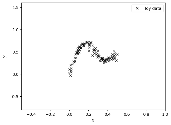
# Generate dataset and grid
X = torch.rand(100, 1) * 0.5
x_grid = torch.linspace(-5, 5, 1000).reshape(-1, 1)

# Define function
def target_toy(x, seed):
    torch.manual_seed(seed)
    epsilons = torch.randn(3) * 0.02
    return (
        x + 0.3 * torch.sin(2 * torch.pi * (x + epsilons[0])) +
        0.3 * torch.sin(4 * torch.pi * (x + epsilons[1])) + epsilons[2]
    )

# Generate target values with different seeds
Y = torch.stack([target_toy(x, seed) for x, seed in zip(X, range(X.shape[0]))])


# Plot the generated data
plt.figure()  # figsize=[12,6], dpi=200)
plt.plot(X, Y, "kx", label="Toy data", alpha=0.8)
# plt.title('Simple 1D example with toy data by Blundell et. al (2015)')
plt.xlabel("$x$")
plt.ylabel("$y$")
plt.xlim(-0.5, 1.0)
plt.ylim(-0.8, 1.6)
plt.legend()
plt.show()

../../_images/tutorials_02_Uncertainty_Quantification_prior_3_0.png

Model

In our implementation of a prior network, we opted to create two sets of parameters for every trained model, \(\theta_{prior}\) and \(\theta_{trainable}\). \(\theta_{prior}\) is randomly initialized and left alone during the training process. This is done because the randomly initialized parameters of the prior network represent our prior beliefs, and we will use these parameters in our forward pass calculations. \(\theta_{trainable}\) will be optimized with an Adam optimizer for mean square error loss. On a forward pass, the prior networks weights \(\theta_{prior}\) will be multiplied by a hyperparameter \(\beta\) that controls how biased our predictions are toward the prior. Then the trainable networks parameters, \(\theta_{trainable}\) are added. This acts as a form of regularization, causing each model to be biased toward a specific prior. When utilzied within an ensemble this be utilized to quantify data uncertainty. In areas with high data uncertainty, the prior \(\theta_{prior}\) should have an extreme influence on predictions due to the trainable parameters not having enough data in that region. In areas with low data uncertainty, the trainable weights \(\theta_{trainable}\) should have an extreme influence on predictions.

\(\theta_{priornet}\) = \(\beta * \theta_{prior} + \theta_{trainable}\)

[2]:

class GenericNet(nn.Module):
    def __init__(self, input_dim):
        super(GenericNet, self).__init__()
        self.input_dim = input_dim

        self.net = nn.Sequential(
            nn.Linear(in_features=input_dim, out_features=16),
            nn.ELU(),
            nn.Linear(in_features=16, out_features=16),
            nn.ELU(),
            nn.Linear(in_features=16, out_features=1)
        )
        # Additional layers can be added here based on the architecture
        # Apply Xavier uniform initialization to the weights
        self.init_weights(self.net)

    def forward(self, x):
        return self.net(x)

    def init_weights(self, m):
        if isinstance(m, nn.Linear):
            nn.init.xavier_uniform_(m.weight)
            m.bias.data.fill_(0.01)


class PriorNet(nn.Module):
    def __init__(self, beta):
        super(PriorNet, self).__init__()
        self.prior = GenericNet(input_dim=1)  # Specify the input dimension
        self.trainable = GenericNet(input_dim=1)  # Specify the input dimension
        self.beta = beta

    def forward(self, x):
        x1 = self.prior(x)
        x2 = self.trainable(x)
        return self.beta * x1 + x2

Training

[3]:

# Function to create train state with key initialization
def create_train_optim(model, lr):
    model.train()  # Set the model in training mode
    optimizer = optim.Adam(model.trainable.parameters(), lr=lr)
    return optimizer

# Training function
def train(model, optimizer, epochs, X, Y):
    for epoch in range(epochs):
        optimizer.zero_grad()
        output = model(X)
        loss = torch.mean((output - Y)**2)
        loss.backward()
        optimizer.step()
    return model

# Prediction function
def get_predictions(model, X):
    model.eval()
    with torch.no_grad():
        Y_prior = model.prior(X)
        Y_trainable = model.trainable(X)
        Y_model = model(X)
    return Y_prior, Y_trainable, Y_model


# Create model and optimizer
beta = 3
lr = 0.03
epochs = 500
# Set a random seed for reproducibility
seed = 2

# Create model and optimizer
torch.manual_seed(seed)
model = PriorNet(beta=beta)
optimizer = create_train_optim(model, lr=lr)

# Train the model
model = train(model, optimizer, epochs=epochs, X=X, Y=Y)

# Get predictions
# predictions = get_predictions(model, beta=3, X=X)
Y_prior, Y_trainable, Y_model = get_predictions(model, x_grid)

Visualizing

[4]:

# Plot the results
plt.figure()  # figsize=[12,6], dpi=200)
plt.plot(X, Y, "kx", label="Toy data", alpha=0.8)
plt.plot(x_grid, 3 * Y_prior, label="prior net (p)")
plt.plot(x_grid, Y_trainable, label="trainable net (t)")
plt.plot(x_grid, Y_model, label="resultant (g)")
# plt.title('Predictions of the prior network: random function')
plt.xlabel("$x$")
plt.ylabel("$y$")
plt.xlim(-0.5, 1.0)
plt.ylim(-0.6, 1.4)
plt.legend()

# plt.savefig("randomized_priors_single_model.pdf")
# plt.savefig("randomized_priors_single_model.png")

plt.show()

../../_images/tutorials_02_Uncertainty_Quantification_prior_10_0.png

[5]:

import torch
from torch.utils.data import DataLoader, TensorDataset
import push.bayes.ensemble
import push.bayes.stein_vgd
import push.bayes.swag

# Constants
N_ENSEMBLES = 8
PRETRAIN_EPOCHS = 250
SWAG_EPOCHS = 250
EPOCHS = 500
NUM_DEVICES = 2
BATCH_SIZE = 100
LEARNING_RATE = 0.03
LEARNING_RATE_SVGD = 0.03
LENGTHSCALE = 0.25
BETA_VALUES = [0.1, 0.2, 0.4, 0.8, 1.6, 3.2, 6.4, 12.8]

# Dataset and DataLoader setup
dataset = TensorDataset(X, Y)
train_loader = DataLoader(dataset, batch_size=BATCH_SIZE, shuffle=True)

# Dictionaries to store results
ensemble_results = {}
swag_results = {}



# Train models without priors
generic_ensemble = push.bayes.ensemble.train_deep_ensemble(
    train_loader,
    torch.nn.MSELoss(),
    EPOCHS,
    GenericNet, 1,
    lr=LEARNING_RATE,
    num_devices=NUM_DEVICES,
    num_ensembles=N_ENSEMBLES
)

generic_swag = push.bayes.swag.train_mswag(
    train_loader,
    torch.nn.MSELoss(),
    PRETRAIN_EPOCHS,
    SWAG_EPOCHS,
    GenericNet, 1,
    num_devices=NUM_DEVICES,
    num_models=N_ENSEMBLES,
    lr=LEARNING_RATE,
    mswag_state={}
)


# Train models with priors using different beta values
for beta in BETA_VALUES:

    prior_ensemble = push.bayes.ensemble.train_deep_ensemble(
        train_loader,
        torch.nn.MSELoss(),
        EPOCHS,
        PriorNet, beta,
        lr=LEARNING_RATE,
        num_devices=NUM_DEVICES,
        num_ensembles=N_ENSEMBLES,
        prior=True
    )
    prior_swag = push.bayes.swag.train_mswag(
        train_loader,
        torch.nn.MSELoss(),
        PRETRAIN_EPOCHS,
        SWAG_EPOCHS,
        PriorNet, beta,
        num_devices=NUM_DEVICES,
        num_models=N_ENSEMBLES,
        lr=LEARNING_RATE,
        prior=True,
        mswag_state={}
    )


    # Save predictions for each beta value
    ensemble_results[beta] = prior_ensemble.posterior_pred(x_grid, f_reg=True, mode=["mean", "std", "pred"])
    swag_results[beta] = prior_swag.posterior_pred(x_grid, f_reg=True, mode=["mean", "std", "pred"])

100%|██████████| 500/500 [00:12<00:00, 40.40it/s, loss=tensor(0.0027)]
100%|██████████| 250/250 [00:05<00:00, 46.35it/s, loss=tensor(0.0078)]
100%|██████████| 250/250 [00:08<00:00, 27.78it/s, loss=tensor(0.0033)]
100%|██████████| 500/500 [00:15<00:00, 32.97it/s, loss=tensor(0.0029)]
100%|██████████| 250/250 [00:06<00:00, 38.32it/s, loss=tensor(0.0060)]
100%|██████████| 250/250 [00:12<00:00, 20.79it/s, loss=tensor(0.0026)]
100%|██████████| 500/500 [00:15<00:00, 32.24it/s, loss=tensor(0.0049)]
100%|██████████| 250/250 [00:06<00:00, 37.72it/s, loss=tensor(0.0060)]
100%|██████████| 250/250 [00:12<00:00, 20.83it/s, loss=tensor(0.0026)]
100%|██████████| 500/500 [00:15<00:00, 32.26it/s, loss=tensor(0.0055)]
100%|██████████| 250/250 [00:06<00:00, 37.96it/s, loss=tensor(0.0059)]
100%|██████████| 250/250 [00:12<00:00, 20.67it/s, loss=tensor(0.0026)]
100%|██████████| 500/500 [00:15<00:00, 32.53it/s, loss=tensor(0.0061)]
100%|██████████| 250/250 [00:06<00:00, 37.77it/s, loss=tensor(0.0059)]
100%|██████████| 250/250 [00:12<00:00, 20.48it/s, loss=tensor(0.0026)]
100%|██████████| 500/500 [00:15<00:00, 32.17it/s, loss=tensor(0.0058)]
100%|██████████| 250/250 [00:06<00:00, 37.95it/s, loss=tensor(0.0058)]
100%|██████████| 250/250 [00:11<00:00, 20.93it/s, loss=tensor(0.0026)]
100%|██████████| 500/500 [00:15<00:00, 32.55it/s, loss=tensor(0.0025)]
100%|██████████| 250/250 [00:06<00:00, 38.56it/s, loss=tensor(0.0055)]
100%|██████████| 250/250 [00:12<00:00, 20.38it/s, loss=tensor(0.0025)]
100%|██████████| 500/500 [00:15<00:00, 31.91it/s, loss=tensor(0.0026)]
100%|██████████| 250/250 [00:06<00:00, 37.87it/s, loss=tensor(0.0059)]
100%|██████████| 250/250 [00:12<00:00, 20.29it/s, loss=tensor(0.0028)]
100%|██████████| 500/500 [00:15<00:00, 32.18it/s, loss=tensor(0.0026)]
100%|██████████| 250/250 [00:06<00:00, 37.81it/s, loss=tensor(0.0067)]
100%|██████████| 250/250 [00:12<00:00, 20.39it/s, loss=tensor(0.0033)]

[6]:

generic_ensemble_output=generic_ensemble.posterior_pred(x_grid, f_reg=True, mode=["mean", "std", "pred"])
generic_swag_output=generic_swag.posterior_pred(x_grid, f_reg=True, mode=["mean", "std", "pred"])

[16]:

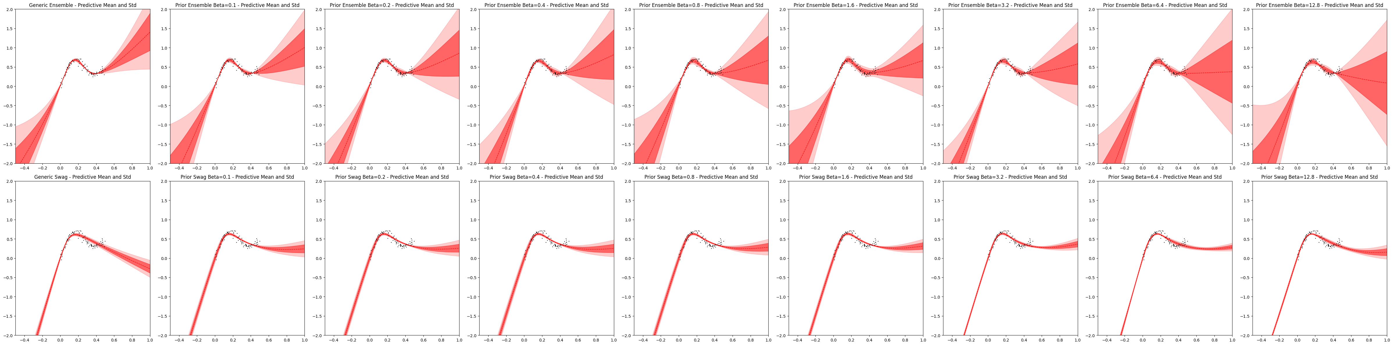
import matplotlib.pyplot as plt
import torch

def plot(outputs, title, axs, col_start):
    # Ensemble outputs
    axs[col_start].plot(X, Y, "kx", label="Toy data", markersize=1)
    axs[col_start].set_xlim(-0.5, 1)
    axs[col_start].set_ylim(-2, 2)
    axs[col_start].plot(x_grid, outputs["mean"], "r--", linewidth=1)
    axs[col_start].fill_between(x_grid.reshape(1, -1)[0], (outputs["mean"] - outputs["std"]).squeeze(), (outputs["mean"] + outputs["std"]).squeeze(), alpha=0.5, color="red")
    axs[col_start].fill_between(x_grid.reshape(1, -1)[0], (outputs["mean"] + 2 * outputs["std"]).squeeze(), (outputs["mean"] - 2 * outputs["std"]).squeeze(), alpha=0.2, color="red")
    axs[col_start].set_title(f"{title} - Predictive Mean and Std")



def plot_all():
    fig, axs = plt.subplots(nrows=2, ncols=9, figsize=[48, 12])  # Adjust dimensions as needed

    # Plot bootstrapped and non-bootstrapped ensemble and individual models in one row
    plot(generic_ensemble_output, "Generic Ensemble", axs[0, :], 0)
    plot(generic_swag_output, "Generic Swag", axs[1, :], 0)
    for idx, beta in enumerate(BETA_VALUES):
        plot(ensemble_results[beta], "Prior Ensemble Beta=" + str(beta), axs[0, :], idx+1)
        plot(swag_results[beta], "Prior Swag Beta=" + str(beta), axs[1, :], idx+1)

    plt.tight_layout()
    plt.show()

# Call this function to generate all plots
plot_all()

../../_images/tutorials_02_Uncertainty_Quantification_prior_13_0.png

The Kernel crashed while executing code in the current cell or a previous cell.

Please review the code in the cell(s) to identify a possible cause of the failure.

Click <a href='https://aka.ms/vscodeJupyterKernelCrash'>here</a> for more info.

View Jupyter <a href='command:jupyter.viewOutput'>log</a> for further details.

[1] Kevin Murphy. Probabilistic Machine Learning Advanced Topics. Chapter 17. The MIT Press: Adaptive computation and machine learning series (2023). Cambridge, Massachusetts.