Domain Uncertainty
In Domain Uncertainty
In-domain uncertainty represents the uncertainty related to inputs drawn from a distribution believed to be equal to the training data distribution. Thus, any uncertainty from in-domain inputs result from our model’s inability to properly understand an in-domain sample, indicating a design error in our model choice (model uncertainty), or the complexity of the problem (data uncertainty). In this tutorial we train on all the numbers, establishing numbers 0-9 as “in domain”, and test on those same numbers to show in domain uncertainty.
[1]
[1]:
import torch
import copy
import os
from torch.utils.data import DataLoader
import torchvision
from torchvision import datasets, transforms
from experiments.nns.bdl import SelectMNISTDataset

# Define the path to directory containing MNIST
mnist_directory = os.path.abspath(os.path.join(os.path.dirname(os.path.abspath("uncertainty.ipynb")), "..","..","..","..","..","..","..", "/usr/data1/vision/data/"))


# Define a transform to normalize the data
transform = transforms.Compose([transforms.ToTensor(), transforms.Normalize((0.5,), (0.5,))])

# Define numbers in domain
in_domain = [0,1,2,3,4,5,6,7,8,9]

# Load the MNIST training dataset
train_dataset = SelectMNISTDataset(root=mnist_directory, train=True, numbers = in_domain, num_entries_per_digit=1000, transform=transform)
[2]:
import torch
from torch.utils.data import DataLoader
import push.bayes.ensemble
import push.bayes.swag
import push.bayes.stein_vgd
from experiments.nns.lenet.lenet import LeNet

# Create data loaders
batch_size = 1000
train_loader = DataLoader(train_dataset, batch_size=batch_size, shuffle=True)
epochs = 500
lr = 0.01
n = 25

ensemble = push.bayes.ensemble.train_deep_ensemble(
        train_loader,
        torch.nn.CrossEntropyLoss(),
        epochs,
        LeNet,
        num_devices=2,
        num_ensembles=n,
        lr = lr
    )
100%|██████████| 500/500 [2:23:48<00:00, 17.26s/it, loss=tensor(2.3027)]
[3]:
pretrain_epochs = 250
swag_epochs = 250
swag = push.bayes.swag.train_mswag(
    train_loader,
    torch.nn.CrossEntropyLoss(),
    pretrain_epochs,
    swag_epochs,
    LeNet,
    num_devices = 2,
    num_models = n,
    lr = lr
)
100%|██████████| 250/250 [1:07:55<00:00, 16.30s/it, loss=tensor(0.0221)]
100%|██████████| 250/250 [1:13:20<00:00, 17.60s/it, loss=tensor(0.0589)]
[13]:
svgd = push.bayes.stein_vgd.train_svgd(
    train_loader,                       # Dataloader
    torch.nn.CrossEntropyLoss(),        # Loss Fn
    epochs,                             # Epochs
    8,                                  # Number of particles
    LeNet,                              # NN
    lengthscale = 0.5,                  # Lengthscale
    lr = 3e-1,                          # Learning Rate
    num_devices = 2,                    # Number of devices
)
100%|██████████| 500/500 [1:55:56<00:00, 13.91s/it, loss=tensor(0.0075)]
[4]:
test_dataset = SelectMNISTDataset(root=mnist_directory, train=False, numbers = [0,1,2,3,4,5,6,7,8,9], num_entries_per_digit=100, transform=transform)
test_batch_size=100
test_loader = DataLoader(test_dataset, batch_size=test_batch_size, shuffle=False)
[5]:
ensemble_outputs = ensemble.posterior_pred(test_loader, f_reg=False, mode=["mode","logits", "prob", "std"])
[6]:
swag_outputs = swag.posterior_pred(test_loader, f_reg=False, mode=["mode","logits", "prob", "std"])
[15]:
svgd_outputs = svgd.posterior_pred(test_loader, f_reg=False, mode=["mode","logits", "prob", "std"])
[7]:
# Display rotated images
# num_images_to_display =
import matplotlib.pyplot as plt

def get_image(number_to_display, dataloader, batch_size):
    number_to_display = number_to_display
    cur_batch = 0
    idx = 0
    for images, labels in test_loader:
        img = images[idx]
        lbl = labels[idx]
        if cur_batch == number_to_display:
            return img
        cur_batch += 1

number_to_display = 0
img = get_image(number_to_display, test_loader, test_batch_size)
idx_image = test_batch_size * number_to_display
plt.imshow(img.squeeze(), cmap='gray')
[7]:
<matplotlib.image.AxesImage at 0x7fe134d13580>
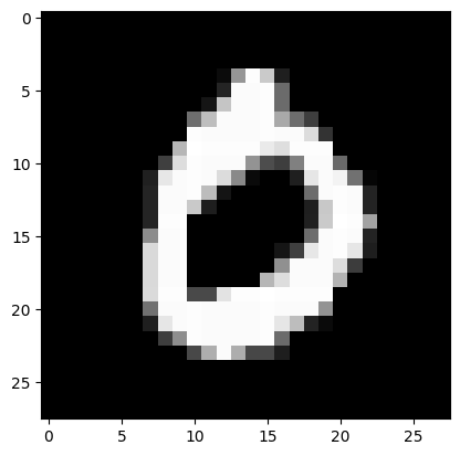
Trained on all numbers, testing on 9
[8]:
import numpy as np
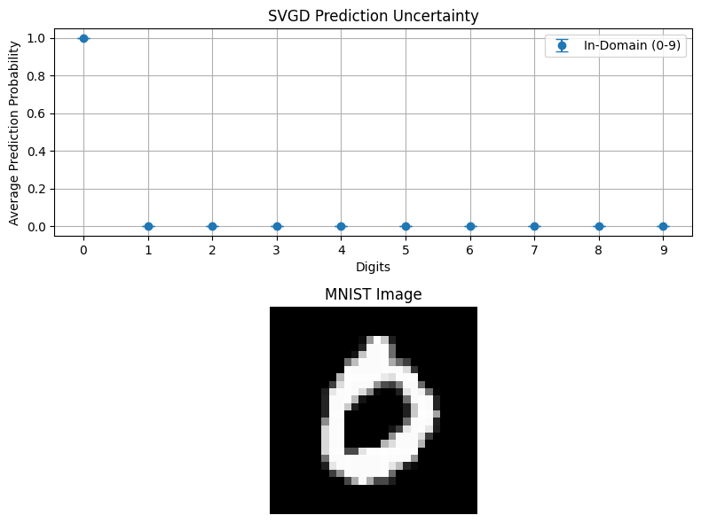
def plot_probabilities(outputs, title):
# Sample average prediction probabilities and standard deviations
digits = np.arange(10) # Digits 0-9
# avg_probs = np.array([0.92, 0.91, 0.93, 0.94, 0.92, 0.95, 0.94, 0.92, 0.93, 0.6]) # Sample average probs
# std_devs = np.array([0.03, 0.02, 0.03, 0.02, 0.03, 0.02, 0.03, 0.03, 0.03, 0.1]) # Sample std devs
plt.figure(figsize=(8, 6))
plt.subplot(2, 1, 1)
# Plotting
plt.errorbar(digits, torch.mean(outputs["prob"], dim=1).squeeze()[idx_image], yerr=outputs["std"][idx_image], fmt='o', capsize=5, label='In-Domain (0-9)')
# plt.scatter(9, 0.6, color='red', label='Out-of-Domain (9)')
plt.xticks(digits)
plt.xlabel('Digits')
plt.ylabel('Average Prediction Probability')
plt.title(title)
plt.legend()
plt.grid(True)
# Second subplot for the MNIST image
plt.subplot(2, 1, 2)
plt.imshow(img.squeeze(), cmap='gray')
plt.axis('off') # Remove axis
plt.title('MNIST Image')
# Adjust layout to prevent overlapping titles
plt.tight_layout()
plt.show()
[9]:
plot_probabilities(ensemble_outputs, "Ensemble Prediction Uncertainty")

[10]:
plot_probabilities(swag_outputs, "SWAG Prediction Uncertainty")

[18]:
plot_probabilities(svgd_outputs, "SVGD Prediction Uncertainty")
Out of Domain Uncertainty
Out of domain uncertainty represents the uncertainty related to inputs drawn from the subspace of unknown data. In this tutorial we examine the MNIST dataset, and train on set of numbers 1-8, establishing our “in-domain” as the numbers 1-8. By testing on the number 9, an out of domain input, we can determine how uncertain our model is when encountering data it is not equipped to handle.
[1]
Dataset
[1]:
import torch
import copy
import os
from torch.utils.data import DataLoader
import torchvision
from torchvision import datasets, transforms
from experiments.nns.bdl import SelectMNISTDataset

# Define the path to directory containing MNIST
mnist_directory = os.path.abspath(os.path.join(os.path.dirname(os.path.abspath("uncertainty.ipynb")), "..","..","..","..","..","..","..", "/usr/data1/vision/data/"))


# Define a transform to normalize the data
transform = transforms.Compose([transforms.ToTensor(), transforms.Normalize((0.5,), (0.5,))])

# Define in and out domain numbers
in_domain = [0,2,4,6,8]
out_domain = [1,3,5,7,9]

# Load the MNIST training dataset
train_dataset = SelectMNISTDataset(root=mnist_directory, train=True, numbers = in_domain, num_entries_per_digit=1000, transform=transform)
[13]:
import torch
from torch.utils.data import DataLoader
import push.bayes.ensemble
from experiments.nns.lenet.lenet import LeNet


# Create data loaders
batch_size = 1000
train_loader = DataLoader(train_dataset, batch_size=batch_size, shuffle=True)
epochs = 500
ensemble = push.bayes.ensemble.train_deep_ensemble(
        train_loader,
        torch.nn.CrossEntropyLoss(),
        epochs,
        LeNet,
        num_devices=2,
        num_ensembles=n,
        cache_size=25,
        lr = lr
    )
100%|██████████| 500/500 [38:13<00:00, 4.59s/it, loss=tensor(0.0146)]
[8]:
pretrain_epochs = 250
swag_epochs = 250
swag = push.bayes.swag.train_mswag(
    train_loader,
    torch.nn.CrossEntropyLoss(),
    pretrain_epochs,
    swag_epochs,
    LeNet,
    num_devices = 2,
    num_models = n,
    lr = lr,
    mswag_state={},
)
100%|██████████| 250/250 [33:41<00:00,  8.09s/it, loss=tensor(0.0060)]
100%|██████████| 250/250 [38:00<00:00,  9.12s/it, loss=tensor(0.0056)]
[6]:
svgd = push.bayes.stein_vgd.train_svgd(
    train_loader,                       # Dataloader
    torch.nn.CrossEntropyLoss(),        # Loss Fn
    epochs,                             # Epochs
    8,                                  # Number of particles
    LeNet,                              # NN
    lengthscale = 0.5,                  # Lengthscale
    lr = 3e-1,                          # Learning Rate
    num_devices = 2,                    # Number of devices
)
100%|██████████| 500/500 [58:15<00:00, 6.99s/it, loss=tensor(0.0050)]
[9]:
test_dataset = SelectMNISTDataset(root=mnist_directory, train=False, numbers = [0,1,2,3,4,5,6,7,8,9], num_entries_per_digit=100, transform=transform)
test_batch_size = 100
test_loader = DataLoader(test_dataset, batch_size=test_batch_size, shuffle=False)
[ ]:
ensemble_outputs = ensemble.posterior_pred(test_loader, f_reg=False, mode=["mode","logits","prob", "std"])
[10]:
swag_outputs = swag.posterior_pred(test_loader, f_reg=False, mode=["mode","logits","prob", "std"])
[8]:
svgd_outputs = svgd.posterior_pred(test_loader, f_reg=False, mode=["mode","logits", "prob", "std"])
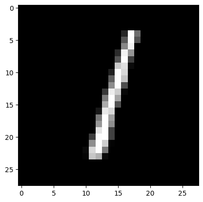
Trained on numbers 0-8, testing on number 9 image
[11]:
# Display rotated images
# num_images_to_display =
import matplotlib.pyplot as plt

def get_image(number_to_display, dataloader, batch_size):
    number_to_display = number_to_display
    cur_batch = 0
    idx = 0
    for images, labels in test_loader:
        img = images[idx]
        lbl = labels[idx]
        if cur_batch == number_to_display:
            return img
        cur_batch += 1

number_to_display = 1
img = get_image(number_to_display, test_loader, test_batch_size)
idx_image = test_batch_size * number_to_display
plt.imshow(img.squeeze(), cmap='gray')
[11]:
<matplotlib.image.AxesImage at 0x7f5e904eaa70>
[12]:
import numpy as np
import matplotlib.pyplot as plt

def plot_probabilities_domain(outputs, title, number, in_domain, out_domain):
    number_to_display = number
    img = get_image(number_to_display, test_loader, test_batch_size)
    idx_image = test_batch_size * number_to_display
    plt.figure(figsize=(8, 6))
    digits = np.arange(10)
    plt.subplot(2, 1, 1)
    # Plotting
    plt.errorbar(in_domain, torch.mean(outputs["prob"], dim=1).squeeze()[idx_image][in_domain], yerr=outputs["std"][idx_image][in_domain], fmt='o', capsize=5, label="In-Domain")
    plt.errorbar(out_domain, torch.mean(outputs["prob"], dim=1).squeeze()[idx_image][out_domain], yerr=outputs["std"][idx_image][out_domain], fmt='o', capsize=5, label ="Out-Domain")

    plt.xticks(digits)
    plt.xlabel('Digits')
    plt.ylabel('Average Prediction Probability')
    plt.title(title)
    plt.legend()
    plt.grid(True)


    # Second subplot for the MNIST image
    plt.subplot(2, 1, 2)
    img = get_image(number_to_display, test_loader, test_batch_size)
    plt.imshow(img.squeeze(), cmap='gray')
    plt.axis('off')  # Remove axis
    plt.title('MNIST Image')

    # Adjust layout to prevent overlapping titles
    plt.tight_layout()

    plt.show()
Out of Sample Predictions
[ ]:
plot_probabilities_domain(ensemble_outputs, "Out of Sample Ensemble Prediction ", out_domain[0], in_domain, out_domain)

[13]:
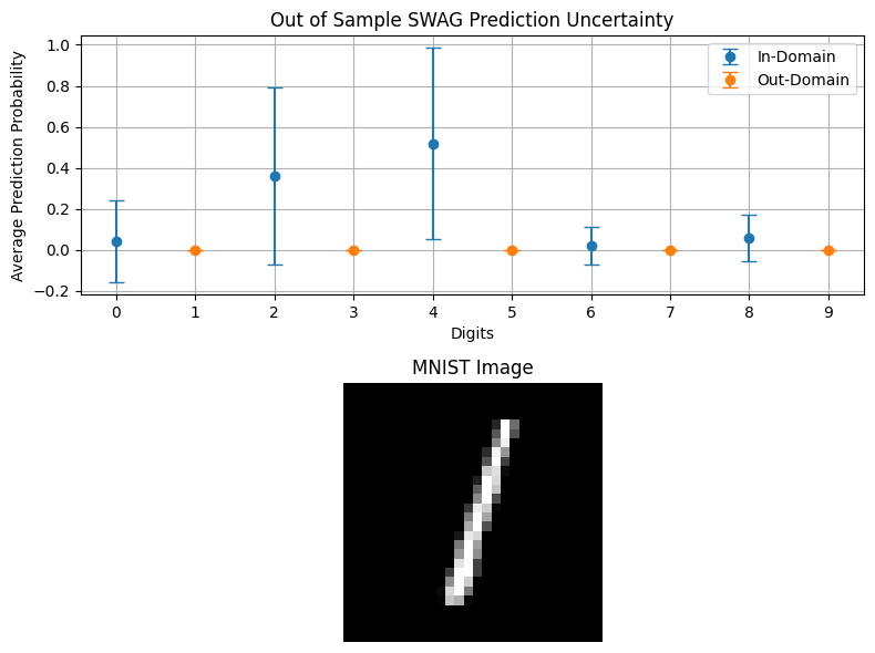
plot_probabilities_domain(swag_outputs, "Out of Sample SWAG Prediction Uncertainty", out_domain[0], in_domain, out_domain)
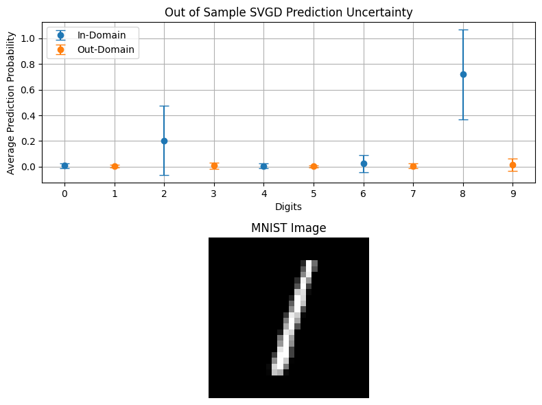
[11]:
plot_probabilities_domain(svgd_outputs, "Out of Sample SVGD Prediction Uncertainty", out_domain[0], in_domain, out_domain)
In Sample Predictions
[ ]:
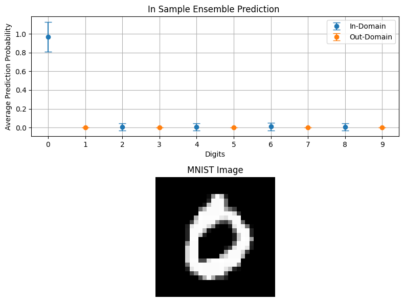
plot_probabilities_domain(ensemble_outputs, "In Sample Ensemble Prediction ", in_domain[0], in_domain, out_domain)
[14]:
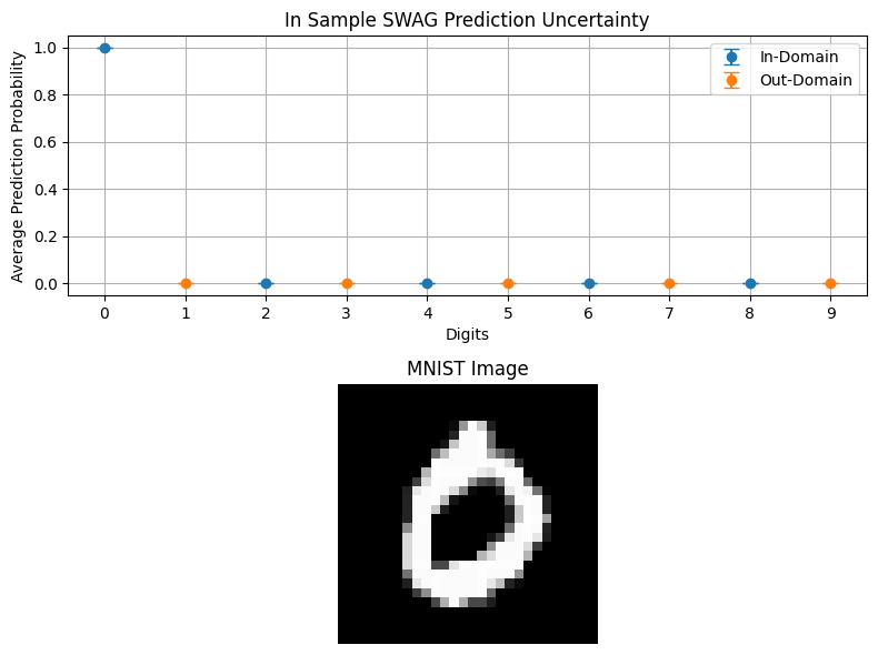
plot_probabilities_domain(swag_outputs, "In Sample SWAG Prediction Uncertainty", in_domain[0], in_domain, out_domain)
[12]:
plot_probabilities_domain(svgd_outputs, "In Sample SVGD Prediction Uncertainty", in_domain[0], in_domain, out_domain)

We can see that the model’s most probable prediction (4) has a very high degree of uncertainty, demonstrated by its very large standard deviation.
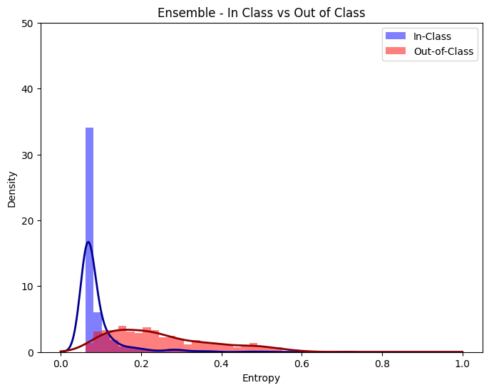
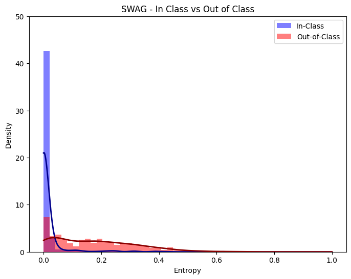
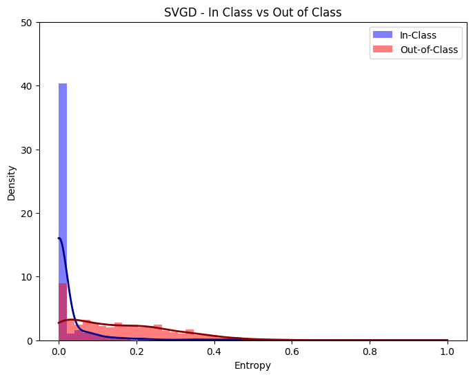
Furthermore, we can visualize the entropy of our predictions for out of domain and in domain samples.
[15]:
import torch
import numpy as np
import matplotlib.pyplot as plt
from scipy.stats import gaussian_kde

def plot_entropy(outputs, title, bins):
    # Define which labels are considered in-class
    in_class_labels = torch.tensor(in_domain)  # Update this list as needed
    # Extract probabilities and predicted classes
    probabilities = outputs['prob']
    filtered_probabilities = probabilities[:, :, in_domain]
    # Calculate predictive entropy for the filtered in-domain probabilities
    # Adjust the calculation to work with the multi-model setup
    entropies = -(filtered_probabilities * torch.log(filtered_probabilities + 1e-10)).sum(dim=2)
    # Average entropy across all models for each sample
    average_entropy = entropies.mean(dim=1)
    # Get true labels (assuming the test_loader has dataset with true labels as the second element)
    true_labels = torch.tensor([label for _, label in test_dataset])
    # # Classify predictions as in-class or out-of-class based on specified labels
    in_class = torch.isin(true_labels, in_class_labels)
    out_of_class = ~in_class
    # # Convert entropy to NumPy for plotting
    entropy_np = average_entropy.numpy()
    entropy_in_class_np = entropy_np[in_class.numpy()]
    entropy_out_of_class_np = entropy_np[out_of_class.numpy()]
    plt.figure(figsize=(8, 6))
    # Adjust your histogram plotting to use the provided bins
    if entropy_in_class_np.size > 0:
        hist_in_class = plt.hist(entropy_in_class_np, bins=bins, density=True, alpha=0.5, color='blue', label='In-Class')
        density_in_class = gaussian_kde(entropy_in_class_np)
        entropy_values_in_class = np.linspace(bins.min(), bins.max(), 1000)
        plt.plot(entropy_values_in_class, density_in_class(entropy_values_in_class), color='darkblue', linewidth=2)

    if entropy_out_of_class_np.size > 0:
        hist_out_of_class = plt.hist(entropy_out_of_class_np, bins=bins, density=True, alpha=0.5, color='red', label='Out-of-Class')
        density_out_of_class = gaussian_kde(entropy_out_of_class_np)
        entropy_values_out_of_class = np.linspace(bins.min(), bins.max(), 1000)
        plt.plot(entropy_values_out_of_class, density_out_of_class(entropy_values_out_of_class), color='darkred', linewidth=2)

    # The rest of your plotting code here
    plt.ylim(0, 50)
    plt.xlabel('Entropy')
    plt.ylabel('Density')
    plt.title(title)
    plt.legend()
    plt.show()
# Define bins based on the range of entropies you expect across all models
# For example, if you expect entropies to be within 0 and 5, you can define:
bins = np.linspace(0, 1, 50)  # Adjust the range and number of bins as needed
# Call the function with the defined bins for each set of outputs
[ ]:
plot_entropy(ensemble_outputs, 'Ensemble - In Class vs Out of Class', bins)
[16]:
plot_entropy(swag_outputs, 'SWAG - In Class vs Out of Class', bins)
[23]:
plot_entropy(svgd_outputs, 'SVGD - In Class vs Out of Class', bins)
[ ]:
# import torch
# import numpy as np
# import matplotlib.pyplot as plt
# from scipy.stats import gaussian_kde

# def plot_entropy(outputs, ax, title, bins):
#     # Define which labels are considered in-class
#     in_class_labels = torch.tensor(in_domain)  # Update this list as needed
#     # Extract probabilities and predicted classes
#     probabilities = outputs['prob']
#     filtered_probabilities = probabilities[:, :, in_domain]
#     # Calculate predictive entropy for the filtered in-domain probabilities
#     entropies = -(filtered_probabilities * torch.log(filtered_probabilities + 1e-10)).sum(dim=2)
#     # Average entropy across all models for each sample
#     average_entropy = entropies.mean(dim=1)
#     # Get true labels (assuming the test_loader has dataset with true labels as the second element)
#     true_labels = torch.tensor([label for _, label in test_dataset])
#     # Classify predictions as in-class or out-of-class based on specified labels
#     in_class = torch.isin(true_labels, in_class_labels)
#     out_of_class = ~in_class
#     # Convert entropy to NumPy for plotting
#     entropy_np = average_entropy.numpy()
#     entropy_in_class_np = entropy_np[in_class.numpy()]
#     entropy_out_of_class_np = entropy_np[out_of_class.numpy()]
#     # Adjust your histogram plotting to use the provided bins
#     if entropy_in_class_np.size > 0:
#         ax.hist(entropy_in_class_np, bins=bins, density=True, alpha=0.5, color='blue', label='In-Class')
#         density_in_class = gaussian_kde(entropy_in_class_np)
#         entropy_values_in_class = np.linspace(bins.min(), bins.max(), 1000)
#         ax.plot(entropy_values_in_class, density_in_class(entropy_values_in_class), color='darkblue', linewidth=2)

#     if entropy_out_of_class_np.size > 0:
#         ax.hist(entropy_out_of_class_np, bins=bins, density=True, alpha=0.5, color='red', label='Out-of-Class')
#         density_out_of_class = gaussian_kde(entropy_out_of_class_np)
#         entropy_values_out_of_class = np.linspace(bins.min(), bins.max(), 1000)
#         ax.plot(entropy_values_out_of_class, density_out_of_class(entropy_values_out_of_class), color='darkred', linewidth=2)

#     ax.set_xlabel('Entropy')
#     ax.set_ylabel('Density')
#     ax.set_title(title)
#     ax.legend()

# # Define bins based on the range of entropies you expect across all models
# bins = np.linspace(0, 1, 50)  # Adjust the range and number of bins as needed

# # Set up a single figure with three subplots
# fig, axs = plt.subplots(1, 3, figsize=(21, 6))  # You can adjust the figsize as needed
# plot_entropy(ensemble_outputs, axs[0], 'Ensemble - In Class vs Out of Class', bins)
# plot_entropy(swag_outputs, axs[1], 'SWAG - In Class vs Out of Class', bins)
# plot_entropy(svgd_outputs, axs[2], 'SVGD - In Class vs Out of Class', bins)
# plt.show()
References
[1] Gawlikowski, J., Njieutcheu Tassi, C. R., Ali, M., Lee, J., Humt, M., Feng, J., Kruspe, A., Triebel, R., Jung, P., Roscher, R., Shahzad, M., Yang, W., Bamler, R., & Zhu, X. X. (2022). A Survey of Uncertainty in Deep Neural Networks. arXiv preprint arXiv:2107.03342.
[2] Maddox, W. J., Garipov, T., Izmailov, P., Vetrov, D., & Wilson, A. G. (2019). A simple baseline for Bayesian uncertainty in deep learning. In Proceedings of the 33rd Conference on Neural Information Processing Systems (NeurIPS 2019) (pp. [20]). Vancouver, Canada: New York University; Samsung AI Center Moscow; Samsung-HSE Laboratory, National Research University Higher School of Economics.